
Blog 3
Blog Post 3: Identify Fakes News.
In this blog, we aim to use machine learning techniques to build a model which can identify fakes news online. We break the modeling process into several parts:
- Obtain training data
- Make a Dataset
- Construct Models
- Model Evaluation
- Embedding Visualization
# Before we start coding, we first import all packages that we need.
import numpy as np
import pandas as pd
import tensorflow as tf

import re
import string

from tensorflow.keras import layers
from tensorflow.keras import losses
from tensorflow import keras

from tensorflow.keras.layers.experimental.preprocessing import TextVectorization
from tensorflow.keras.layers.experimental.preprocessing import StringLookup

from matplotlib import pyplot as plt

from sklearn.decomposition import PCA
import plotly.express as px
Step1: Acquire Training Data
We first retrieve the dataset by using pd.read_csv() to read in the online csv file directly into a dateframe.
Remark on data file: each row is an individual instance of news, which includes the title and the text of the news. The value in the fake column informs us whether this piece of news is fake or not. Fake = 1 indicates the news is fake, while Fake = 0 means the news is true.
train_url = "https://github.com/PhilChodrow/PIC16b/blob/master/datasets/fake_news_train.csv?raw=true"
df = pd.read_csv(train_url)
df
| Unnamed: 0 | title | text | fake | |
|---|---|---|---|---|
| 0 | 17366 | Merkel: Strong result for Austria's FPO 'big c... | German Chancellor Angela Merkel said on Monday... | 0 |
| 1 | 5634 | Trump says Pence will lead voter fraud panel | WEST PALM BEACH, Fla.President Donald Trump sa... | 0 |
| 2 | 17487 | JUST IN: SUSPECTED LEAKER and “Close Confidant... | On December 5, 2017, Circa s Sara Carter warne... | 1 |
| 3 | 12217 | Thyssenkrupp has offered help to Argentina ove... | Germany s Thyssenkrupp, has offered assistance... | 0 |
| 4 | 5535 | Trump say appeals court decision on travel ban... | President Donald Trump on Thursday called the ... | 0 |
| ... | ... | ... | ... | ... |
| 22444 | 10709 | ALARMING: NSA Refuses to Release Clinton-Lynch... | If Clinton and Lynch just talked about grandki... | 1 |
| 22445 | 8731 | Can Pence's vow not to sling mud survive a Tru... | () - In 1990, during a close and bitter congre... | 0 |
| 22446 | 4733 | Watch Trump Campaign Try To Spin Their Way Ou... | A new ad by the Hillary Clinton SuperPac Prior... | 1 |
| 22447 | 3993 | Trump celebrates first 100 days as president, ... | HARRISBURG, Pa.U.S. President Donald Trump hit... | 0 |
| 22448 | 12896 | TRUMP SUPPORTERS REACT TO DEBATE: “Clinton New... | MELBOURNE, FL is a town with a population of 7... | 1 |
22449 rows × 4 columns
Step2: Contruct the Dataset
Before we train our model on it, we need to first clean the data. There are non-important words in the texts and titles. For example, the word “and” does not inform us about the truthfulness of the news. These words are known as the stopwords, so we need to remove them from the dataset.
Luckily, there is a standardized library of stopwords which we can easily import for our own use. This stopword list is from the sklearn.feature_xtraction module.
# import the stopwords library
from sklearn.feature_extraction import text
stop = text.ENGLISH_STOP_WORDS
# now "stop" contains the list of stopwords that we wish to remove from the data.
# we thus remove all stopwords by using lambda expression and .apply method
df['text'] = df['text'].apply(lambda x: ' '.join([word for word in x.split() if word.lower() not in (stop)]))
df['title'] = df['title'].apply(lambda x: ' '.join([word for word in x.split() if word.lower() not in (stop)]))
df
| Unnamed: 0 | title | text | fake | |
|---|---|---|---|---|
| 0 | 17366 | Merkel: Strong result Austria's FPO 'big chall... | German Chancellor Angela Merkel said Monday st... | 0 |
| 1 | 5634 | Trump says Pence lead voter fraud panel | WEST PALM BEACH, Fla.President Donald Trump sa... | 0 |
| 2 | 17487 | JUST IN: SUSPECTED LEAKER “Close Confidant” Ja... | December 5, 2017, Circa s Sara Carter warned m... | 1 |
| 3 | 12217 | Thyssenkrupp offered help Argentina disappeare... | Germany s Thyssenkrupp, offered assistance Arg... | 0 |
| 4 | 5535 | Trump say appeals court decision travel ban 'p... | President Donald Trump Thursday called appella... | 0 |
| ... | ... | ... | ... | ... |
| 22444 | 10709 | ALARMING: NSA Refuses Release Clinton-Lynch Ta... | Clinton Lynch just talked grandkids secret tra... | 1 |
| 22445 | 8731 | Pence's vow sling mud survive Trump campaign? | () - 1990, close bitter congressional race, Mi... | 0 |
| 22446 | 4733 | Watch Trump Campaign Try Spin Way ‘I Love War’... | new ad Hillary Clinton SuperPac Priorities USA... | 1 |
| 22447 | 3993 | Trump celebrates 100 days president, blasts media | HARRISBURG, Pa.U.S. President Donald Trump hit... | 0 |
| 22448 | 12896 | TRUMP SUPPORTERS REACT DEBATE: “Clinton News N... | MELBOURNE, FL town population 76,000. Trump he... | 1 |
22449 rows × 4 columns
We then transform the dataframe into a dataset object that can be correctly handled by tensorflow(the machine learning package we use).
 data = tf.data.Dataset.from_tensor_slices(
            ({
                    "title" : df[["title"]],
                    "text" : df[["text"]]
                }, {
                    "fake" : df[["fake"]]
                }))
We can combine the cleaning process and the transforming process together by writing a function that takes inputs of the dataframe and return the ideal data set
def make_dataset(df):
    """
    A function that creates a fakenews tf.data.Dataset from a dataframe after cleaning all stopwords
    It will also add a batch configue to the returned dataset, the size of batches being 100

    input: df, pd.DataFrame object
    output: tf.data.Dataset with batch_size 100
    """
    # Excluding the stopwords from the dataframe
    stop = text.ENGLISH_STOP_WORDS
    df['text'] = df['text'].apply(lambda x: ' '.join([word for word in x.split() if word.lower() not in (stop)]))
    df['title'] = df['title'].apply(lambda x: ' '.join([word for word in x.split() if word.lower() not in (stop)]))

    # Convert the dataframe into the Dataset object in tensorflow
    # Here, we need to tell tensorflow which columns are the inputs ("text", "title") and which column is the desired out ("fake")
    data = tf.data.Dataset.from_tensor_slices(
            ({
                    "title" : df[["title"]],
                    "text" : df[["text"]]
                }, {
                    "fake" : df[["fake"]]
                }))

    # We set the dataset batch size to 100
    # This means when we train our model, it will take one batch each time
    # And will not loop over the entire 20000+ rows every time
    data = data.batch(100)
    return data
# We create the dataset using the above defined function
data = make_dataset(df)
I gave suggestions to one of my peers to potentially use lambda function instead of writing a function on your own to shorten the length of code.
To train the model, we do train-test-split. The tf.data.Dataset has built-in methods that will allow us to do this. We will leave out 20% of the data for validation purpose.
Since the dataset is shuffled already, we will not do the split randomly
train_size = int(0.8*len(data))
val_size   = int(0.2*len(data))

# The take(n method allows us to take the first n 'rows'
train = data.take(train_size)
# And the skip method allows us to ignore the first n 'rows' and take the rest
val   = data.skip(train_size).take(val_size)

# Check the length of the train and test dataset
len(train), len(val)
(180, 45)
Step3: Construct Models Now we have the data to build the model. Since we are given both text and title in the dataframe, we might wonder which one will help us more when we want to identify the fake news. So we are going to create three models in this part:
- Model 1 only uses information from the article titles;
- Model 2 only uses information from the article texts;
- Model 3 uses both.
Then we evaluate how each model performs and see which one might perform better.
Remark: Before we construct different models, we have last steps to do– standardization and vectorization. Because the models will not be able directly comprehend words, what matters is actually the frequency of the words in the dataset. To make the machine understand the text data, we need to do the vectorization. We have buildt-in function from tensorflow that will help as to achieve this.
# We first specify the maximum number of different words we want to consider
# We are only going to look at the 2000 words which appear most frequently in the texts/titles
size_vocabulary = 2000

# The first step in vectorization is to standardize the texts/titles
# We are going to make all words appear in lower cases, and we will drop all the punctuations
# After we define the function, tensorflow will automatically apply it when necessary
def standardization(input_data):
    """
    A standardization function that converts all letters to lower cases and drop punctuations

    input: tf.data.Dataset object
    ouput: the same dataset in lower case with no punctuations
    """
    lowercase = tf.strings.lower(input_data)
    no_punctuation = tf.strings.regex_replace(lowercase,
                        '[%s]' % re.escape(string.punctuation),'')
    return no_punctuation


# Then we can use vectorization layer from tensorflow to vectorize the standardized data
# Pass the size_vocabulary and the standardization function to it
def make_vectorization_layer():
    vectorize_layer = TextVectorization(
    standardize=standardization, # automatically apply the standardization function
    max_tokens=size_vocabulary, # only consider this amount of words
    output_mode='int',
    output_sequence_length=500)
    return vectorize_layer

# Then we are ready to build the models
Model1: Only the Article Title as an input
The model we are going to build will be a bunch of layers stacked on top of each other. For example, we first pass our dataset to a vectorization layer that vectorizes the strings. Then another layer that does the embedding. And then some other layers to identify the important words and features, etc. Here, we first create a vectorization layer using the function we defined above. Because we are using only the information from the titles, so we adapt the vectorization layer using only the title column of the dataset.
vectorize_layer1 = make_vectorization_layer()
vectorize_layer1.adapt(train.map(lambda x, y: x["title"]))
For the model to know where to start, we will have to tell is what kind of input it should accept. In this case, it’s a one-column single input, and we give this particular input the name title. Here we are not passing the title column to the model yet, and this is just a promise that we will pass it something as specified here.
title_input = keras.Input(
    shape = (1,),
    name = "title",
    dtype = "string"
)
Model output would have different layers to deal with the input, vectorize it, do the embedding and identify the features/important words and finally produce its prediction. The layer module form tensorflow help us handle it.
# First, let's include the vectorizaion layer we definied above
title_features = vectorize_layer1(title_input)
# Then an embedding layer. We use dimension = 10 for the model
title_features = layers.Embedding(size_vocabulary, 10, name = "embedding_title")(title_features)
# Drop 20% of the indicators to avoid overfitting
title_features = layers.Dropout(0.2)(title_features)
# Consolidate the features using GlobalAveragePooling
title_features = layers.GlobalAveragePooling1D()(title_features)
# Drop again to avoid overfitting
title_features = layers.Dropout(0.2)(title_features)
# Pass it to a Dense Layer to do feature identification
title_features = layers.Dense(32, activation='relu')(title_features)
# Output the result, because we are dealing with 2 cases: true and false
# thus, the output whould have exactly two units
title_features = layers.Dense(2, name = "fake")(title_features)
# Then we make a model with the specified input and output
model1 = keras.Model(
    inputs = [title_input],
    outputs = title_features
)
# we can check the model structure
model1.summary()
Model: "model"
_________________________________________________________________
Layer (type)                 Output Shape              Param #
=================================================================
title (InputLayer)           [(None, 1)]               0
_________________________________________________________________
text_vectorization (TextVect (None, 500)               0
_________________________________________________________________
embedding_title (Embedding)  (None, 500, 10)           20000
_________________________________________________________________
dropout (Dropout)            (None, 500, 10)           0
_________________________________________________________________
global_average_pooling1d (Gl (None, 10)                0
_________________________________________________________________
dropout_1 (Dropout)          (None, 10)                0
_________________________________________________________________
dense (Dense)                (None, 32)                352
_________________________________________________________________
fake (Dense)                 (None, 2)                 66
=================================================================
Total params: 20,418
Trainable params: 20,418
Non-trainable params: 0
_________________________________________________________________
Then we need to complie and run the model. For simplicity, we will use the most traditional optimizer “adam” and a standard loss function for category identification “SparseCategoricalCrossentropy” . The metric accuracy means if we are making the right prediction or not.
model1.compile(optimizer = "adam",
              loss = losses.SparseCategoricalCrossentropy(from_logits=True),
              metrics=['accuracy']
)
history = model1.fit(train,
            validation_data = val,
            epochs = 15, # we train the model 15 times using 15 different batches from the dataset
            verbose = True)
Epoch 1/15


/usr/local/lib/python3.7/dist-packages/tensorflow/python/keras/engine/functional.py:591: UserWarning:

Input dict contained keys ['text'] which did not match any model input. They will be ignored by the model.


180/180 [==============================] - 3s 15ms/step - loss: 0.6918 - accuracy: 0.5182 - val_loss: 0.6900 - val_accuracy: 0.5266
Epoch 2/15
180/180 [==============================] - 2s 14ms/step - loss: 0.6853 - accuracy: 0.5542 - val_loss: 0.6725 - val_accuracy: 0.5293
Epoch 3/15
180/180 [==============================] - 2s 14ms/step - loss: 0.6214 - accuracy: 0.7509 - val_loss: 0.5343 - val_accuracy: 0.8568
Epoch 4/15
180/180 [==============================] - 3s 15ms/step - loss: 0.4377 - accuracy: 0.8619 - val_loss: 0.3555 - val_accuracy: 0.8757
Epoch 5/15
180/180 [==============================] - 2s 14ms/step - loss: 0.3071 - accuracy: 0.8908 - val_loss: 0.2723 - val_accuracy: 0.8921
Epoch 6/15
180/180 [==============================] - 2s 13ms/step - loss: 0.2452 - accuracy: 0.9104 - val_loss: 0.2275 - val_accuracy: 0.9049
Epoch 7/15
180/180 [==============================] - 2s 13ms/step - loss: 0.2113 - accuracy: 0.9208 - val_loss: 0.1964 - val_accuracy: 0.9227
Epoch 8/15
180/180 [==============================] - 2s 14ms/step - loss: 0.1875 - accuracy: 0.9300 - val_loss: 0.1799 - val_accuracy: 0.9292
Epoch 9/15
180/180 [==============================] - 2s 14ms/step - loss: 0.1711 - accuracy: 0.9358 - val_loss: 0.1669 - val_accuracy: 0.9341
Epoch 10/15
180/180 [==============================] - 3s 14ms/step - loss: 0.1589 - accuracy: 0.9390 - val_loss: 0.1604 - val_accuracy: 0.9341
Epoch 11/15
180/180 [==============================] - 3s 15ms/step - loss: 0.1505 - accuracy: 0.9426 - val_loss: 0.1551 - val_accuracy: 0.9355
Epoch 12/15
180/180 [==============================] - 3s 15ms/step - loss: 0.1443 - accuracy: 0.9447 - val_loss: 0.1493 - val_accuracy: 0.9384
Epoch 13/15
180/180 [==============================] - 3s 14ms/step - loss: 0.1357 - accuracy: 0.9481 - val_loss: 0.1465 - val_accuracy: 0.9391
Epoch 14/15
180/180 [==============================] - 3s 15ms/step - loss: 0.1312 - accuracy: 0.9494 - val_loss: 0.1428 - val_accuracy: 0.9411
Epoch 15/15
180/180 [==============================] - 3s 14ms/step - loss: 0.1298 - accuracy: 0.9492 - val_loss: 0.1411 - val_accuracy: 0.9407
As we train the model multiple times, we see that the accuracy gradually grows.We can visualize the accuracy over time using plotly.
plt.plot(history.history["accuracy"], label = "Training")
plt.plot(history.history["val_accuracy"], label = "Validations")
plt.savefig("model1.jpg")
plt.legend()
<matplotlib.legend.Legend at 0x7fdf3e0c0890>
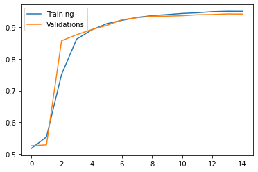
We see that though the accuracy on the training data is likely to increase, the accuracy on the validation dataset may not. This suggests that we might overfit the data if we do more training on the model, so we will stop here. The model with only title as input has 95% accuracy on the training dataset with a nearly 94% accuracy on the validation dataset, which is acceptable.
Some of my peers suggested to use a vectorization layer for all three models, but I feel like making a vectorization layer for each of the three models might be better so I did not shorten the code.
Model 2: Only the Article Texts as Input
Then, we will follow the same process to create our second model, but this time, we are only using the text part of the dataset.
# Second vectorization layer only with the text part
vectorize_layer2 = make_vectorization_layer()
vectorize_layer2.adapt(train.map(lambda x, y: x["text"]))
# A single input using only the texts
text_input = keras.Input(
    shape = (1,),
    name = "text",
    dtype = "string"
)
# First, let's include the vectorizaion layer we definied above
text_features = vectorize_layer2(text_input)
# First, let's include the vectorizaion layer we definied above
text_features = layers.Embedding(size_vocabulary, 10, name = "embedding_text")(text_features)
# Drop 20% of the indicators to avoid overfitting
text_features = layers.Dropout(0.2)(text_features)
# Let's consolidate the features using GlobalAveragePooling
text_features = layers.GlobalAveragePooling1D()(text_features)
# Drop again to avoid overfitting
text_features = layers.Dropout(0.2)(text_features)
# We pass it to a Dense Layer to do feature identification
text_features = layers.Dense(32, activation='relu')(text_features)
# Output the result, because we are dealing with 2 cases: true and false
text_features = layers.Dense(2, name = "fake")(text_features)
# Declare the model
model2 = keras.Model(
    inputs = text_input,
    outputs = text_features
)
# Take a look at the model structure
model2.summary()
Model: "model_1"
_________________________________________________________________
Layer (type)                 Output Shape              Param #
=================================================================
text (InputLayer)            [(None, 1)]               0
_________________________________________________________________
text_vectorization_1 (TextVe (None, 500)               0
_________________________________________________________________
embedding_text (Embedding)   (None, 500, 10)           20000
_________________________________________________________________
dropout_2 (Dropout)          (None, 500, 10)           0
_________________________________________________________________
global_average_pooling1d_1 ( (None, 10)                0
_________________________________________________________________
dropout_3 (Dropout)          (None, 10)                0
_________________________________________________________________
dense_1 (Dense)              (None, 32)                352
_________________________________________________________________
fake (Dense)                 (None, 2)                 66
=================================================================
Total params: 20,418
Trainable params: 20,418
Non-trainable params: 0
_________________________________________________________________
# Compile our model2
model2.compile(optimizer = "adam",
              loss = losses.SparseCategoricalCrossentropy(from_logits=True),
              metrics=['accuracy']
)
# Train the model
history = model2.fit(train,
            validation_data = val,
            epochs = 15,
            verbose = True)
Epoch 1/15


/usr/local/lib/python3.7/dist-packages/tensorflow/python/keras/engine/functional.py:591: UserWarning:

Input dict contained keys ['title'] which did not match any model input. They will be ignored by the model.


180/180 [==============================] - 5s 22ms/step - loss: 0.6521 - accuracy: 0.6959 - val_loss: 0.5155 - val_accuracy: 0.9326
Epoch 2/15
180/180 [==============================] - 4s 21ms/step - loss: 0.3282 - accuracy: 0.9336 - val_loss: 0.2052 - val_accuracy: 0.9676
Epoch 3/15
180/180 [==============================] - 4s 21ms/step - loss: 0.1678 - accuracy: 0.9634 - val_loss: 0.1323 - val_accuracy: 0.9742
Epoch 4/15
180/180 [==============================] - 4s 21ms/step - loss: 0.1196 - accuracy: 0.9736 - val_loss: 0.1033 - val_accuracy: 0.9773
Epoch 5/15
180/180 [==============================] - 4s 21ms/step - loss: 0.0962 - accuracy: 0.9785 - val_loss: 0.0882 - val_accuracy: 0.9807
Epoch 6/15
180/180 [==============================] - 4s 21ms/step - loss: 0.0799 - accuracy: 0.9819 - val_loss: 0.0779 - val_accuracy: 0.9825
Epoch 7/15
180/180 [==============================] - 4s 21ms/step - loss: 0.0700 - accuracy: 0.9837 - val_loss: 0.0714 - val_accuracy: 0.9836
Epoch 8/15
180/180 [==============================] - 4s 21ms/step - loss: 0.0621 - accuracy: 0.9858 - val_loss: 0.0666 - val_accuracy: 0.9840
Epoch 9/15
180/180 [==============================] - 4s 21ms/step - loss: 0.0545 - accuracy: 0.9874 - val_loss: 0.0637 - val_accuracy: 0.9843
Epoch 10/15
180/180 [==============================] - 4s 21ms/step - loss: 0.0497 - accuracy: 0.9887 - val_loss: 0.0610 - val_accuracy: 0.9847
Epoch 11/15
180/180 [==============================] - 4s 21ms/step - loss: 0.0453 - accuracy: 0.9897 - val_loss: 0.0591 - val_accuracy: 0.9845
Epoch 12/15
180/180 [==============================] - 4s 21ms/step - loss: 0.0402 - accuracy: 0.9907 - val_loss: 0.0598 - val_accuracy: 0.9847
Epoch 13/15
180/180 [==============================] - 4s 21ms/step - loss: 0.0366 - accuracy: 0.9921 - val_loss: 0.0577 - val_accuracy: 0.9863
Epoch 14/15
180/180 [==============================] - 4s 21ms/step - loss: 0.0336 - accuracy: 0.9925 - val_loss: 0.0583 - val_accuracy: 0.9856
Epoch 15/15
180/180 [==============================] - 4s 21ms/step - loss: 0.0308 - accuracy: 0.9933 - val_loss: 0.0585 - val_accuracy: 0.9861
This model has better accuracy! We visualize the accuracy over time.
plt.plot(history.history["accuracy"],label = "Training")
plt.plot(history.history["val_accuracy"],label = "Validations")
plt.legend()
plt.savefig("model2.jpg")
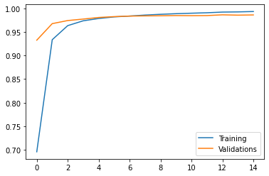
Similarly, though the accuracy on the training data is likely to increase, the accuracy on the validation dataset may not, which aslo suggests that we might overfit the data if do more training on the model. So we will stop here. The model has 99.3% accuracy on the training dataset and a nearly 98.6% accuracy on the validation dataset. Seems awesome!
Model3: Input Both Ariticle Texts and Titles
In the last model, we will incorporate both the text and the title and build the model!
# our 3rd vectorization layer, and this time feed it with both titles and texts
vectorize_layer3 = make_vectorization_layer()
vectorize_layer3.adapt(train.map(lambda x, y: x["title"]))
vectorize_layer3.adapt(train.map(lambda x, y: x["text"]))
In this model, we are going to construct a model that has two parts, one dealing with the title and the other part dealing with the texts, we will combine both parts afterwards and make the right prediction.
I got a great suggeston from my peers that I should also use epoch = 15 in the 3rd model because I have used epoch = 15 in the previous two models. Epochs should be same to make fair comparisons.
embedding_layer = layers.Embedding(size_vocabulary, 10, name = "embedding")
text_features = vectorize_layer3(text_input)
text_features = embedding_layer(text_features)
text_features = layers.Dropout(0.2)(text_features)
text_features = layers.GlobalAveragePooling1D()(text_features)
text_features = layers.Dropout(0.2)(text_features)
text_features = layers.Dense(32, activation='relu')(text_features)
title_features = vectorize_layer3(title_input)
title_features = embedding_layer(title_features)
title_features = layers.Dropout(0.2)(title_features)
title_features = layers.GlobalAveragePooling1D()(title_features)
title_features = layers.Dropout(0.2)(title_features)
title_features = layers.Dense(32, activation='relu')(title_features)
main = layers.concatenate([text_features, title_features], axis = 1)
main = layers.Dropout(0.2)(main)
main = layers.Dense(32, activation='relu')(main)
main = layers.Dropout(0.2)(main)
output = layers.Dense(2, name = "fake")(main)
model3 = keras.Model(
    inputs = [text_input, title_input],
    outputs = output
)
model3.compile(optimizer = "adam",
              loss = losses.SparseCategoricalCrossentropy(from_logits=True),
              metrics=['accuracy']
)
history = model3.fit(train,
          epochs = 15,
          validation_data = val,
          verbose = True)
plt.plot(history.history["accuracy"],label = "Training")
plt.plot(history.history["val_accuracy"],label = "Validations")
plt.legend()
plt.savefig("model3.jpg")
Epoch 1/15
180/180 [==============================] - 7s 31ms/step - loss: 0.6033 - accuracy: 0.6746 - val_loss: 0.2662 - val_accuracy: 0.9557
Epoch 2/15
180/180 [==============================] - 5s 29ms/step - loss: 0.1638 - accuracy: 0.9464 - val_loss: 0.0948 - val_accuracy: 0.9768
Epoch 3/15
180/180 [==============================] - 5s 29ms/step - loss: 0.0934 - accuracy: 0.9722 - val_loss: 0.0701 - val_accuracy: 0.9816
Epoch 4/15
180/180 [==============================] - 5s 29ms/step - loss: 0.0705 - accuracy: 0.9779 - val_loss: 0.0641 - val_accuracy: 0.9847
Epoch 5/15
180/180 [==============================] - 5s 30ms/step - loss: 0.0564 - accuracy: 0.9848 - val_loss: 0.0582 - val_accuracy: 0.9847
Epoch 6/15
180/180 [==============================] - 5s 29ms/step - loss: 0.0486 - accuracy: 0.9861 - val_loss: 0.0556 - val_accuracy: 0.9845
Epoch 7/15
180/180 [==============================] - 5s 30ms/step - loss: 0.0411 - accuracy: 0.9886 - val_loss: 0.0564 - val_accuracy: 0.9843
Epoch 8/15
180/180 [==============================] - 5s 29ms/step - loss: 0.0353 - accuracy: 0.9910 - val_loss: 0.0528 - val_accuracy: 0.9858
Epoch 9/15
180/180 [==============================] - 5s 30ms/step - loss: 0.0327 - accuracy: 0.9917 - val_loss: 0.0555 - val_accuracy: 0.9843
Epoch 10/15
180/180 [==============================] - 5s 30ms/step - loss: 0.0287 - accuracy: 0.9927 - val_loss: 0.0576 - val_accuracy: 0.9843
Epoch 11/15
180/180 [==============================] - 5s 30ms/step - loss: 0.0233 - accuracy: 0.9942 - val_loss: 0.0548 - val_accuracy: 0.9865
Epoch 12/15
180/180 [==============================] - 5s 30ms/step - loss: 0.0217 - accuracy: 0.9952 - val_loss: 0.0731 - val_accuracy: 0.9793
Epoch 13/15
180/180 [==============================] - 5s 29ms/step - loss: 0.0212 - accuracy: 0.9947 - val_loss: 0.0690 - val_accuracy: 0.9847
Epoch 14/15
180/180 [==============================] - 5s 29ms/step - loss: 0.0180 - accuracy: 0.9956 - val_loss: 0.0765 - val_accuracy: 0.9791
Epoch 15/15
180/180 [==============================] - 5s 29ms/step - loss: 0.0170 - accuracy: 0.9958 - val_loss: 0.0778 - val_accuracy: 0.9789
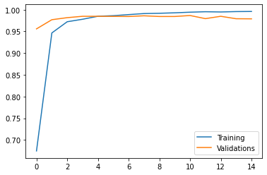
Again, though the accuracy on the training data will likely to increase, the accuracy on the validation dataset will not. This suggests that we might overfit the data if we do more training on the model. The model has 99.6% accuracy on the training dataset with a 98% accuracy on the validation dataset.
Step 4: Evaluating the Results
We see that the second and the thrid model perform relatively better compared to the first one that only considers the title information. Let’s use another validation dataset on the two models and see how they would perform.
#The test dataset can be accessed directly from Professor Chodrow’s github page.
test_url = "https://github.com/PhilChodrow/PIC16b/blob/master/datasets/fake_news_test.csv?raw=true"
de = pd.read_csv(test_url)
# In order to feed data to the models, we need to make it a dataset using the earlier makedata_set function.
test = make_dataset(de)
Let’s first see how the second and third model performs. We use the evaluate method to let the model to predict the labels.
model2.evaluate(test)
225/225 [==============================] - 2s 10ms/step - loss: 0.0634 - accuracy: 0.9827


[0.0633782148361206, 0.9827163815498352]
model3.evaluate(test)
225/225 [==============================] - 3s 12ms/step - loss: 0.0961 - accuracy: 0.9766


[0.09612250328063965, 0.9765691161155701]
It seems that model 2 has a slightly better accuracy, but both models have nearly the same accuracy.
Step 5: Word Embedding PCA
Lastly, we visualize the features Model 3 found: words that are usually associated with fake news and that are associated with accurate news. Tool: We use the PCA module(Principal Component Analysis). It can reduce higher dimensional weights into 1 or 2 dimensional weights to help visualize the results on a 2-D plot.
weights = model3.get_layer('embedding').get_weights()[0] # get the weights from the embedding layer
vocab = vectorize_layer3.get_vocabulary() # get the vocabulary
# Apply PCA on the high-dimensional weights
pca = PCA(n_components=2)
weights = pca.fit_transform(weights)

# Create a dataframe accordingly
# Using the first weight as x value
# And the second weight as y value
embedding_df = pd.DataFrame({
    'word' : vocab,
    'x0'   : weights[:,0],
    'x1'   : weights[:,1]
})
# Plot our word embedding
fig = px.scatter(embedding_df,
          x = "x0",
          y = "x1",
          size = list(np.ones(len(embedding_df))),
          size_max = 2,
          hover_name = "word")

from plotly.io import write_html
write_html(fig, "PCA.html")
fig.show()
Words on the right seem to be relevant to political news: there are words relating to date like “monday”, and other typical words in political news such as “Trump”, “Macron”,”parties”,”europeans”,”chinese”, “religions”. On the left hand side, there are emotinoal words such as “simply”,”extremely”,”bad”,”correct”. It appears to me that political news might just state the fact going on in the world so it might has less possibility to become fake news, so words on the right might be associated with real news.
I got suggestion that I should try to add my personal understanding and interpretation on the plot such as what kinds of words are related to fake news. I think it’s a great suggestion so I add my comments of the plot above.
One of my peer did not strucutre the code in this part very well, so I gave suggestions to one of my peers to make clear explanation on the code and make sure the most relavant two lines of codes are together and not sperated by other codes.