Blog Post 2: Spectral Clustering

In this blog post, you’ll write a tutorial on a simple version of the spectral clustering algorithm for clustering data points. Each of the below parts will pose to you one or more specific tasks. You should plan to both:

Notation

In all the math below:

• Boldface capital letters like $\mathbf{A}$ refer to matrices (2d arrays of numbers).
• Boldface lowercase letters like $\mathbf{v}$ refer to vectors (1d arrays of numbers).
• $\mathbf{A}\mathbf{B}$ refers to a matrix-matrix product (A@B). $\mathbf{A}\mathbf{v}$ refers to a matrix-vector product (A@v).

Introduction

In this problem, we’ll study spectral clustering. Spectral clustering is an important tool for identifying meaningful parts of data sets with complex structure. To start, let’s look at an example where we don’t need spectral clustering.

import numpy as np
from sklearn import datasets
from matplotlib import pyplot as plt

n = 200
np.random.seed(1111)
#n_samples = total number of points equally divided among clusters
#Shuffle the samples.
#cluster_std: The standard deviation of the clusters.
X, y = datasets.make_blobs(n_samples=n, shuffle=True, random_state=None, centers = 2, cluster_std = 2.0)
#Xndarray of shape (n_samples, n_features):The generated samples.
#yndarray of shape (n_samples,):The integer labels for cluster membership of each sample
plt.scatter(X[:,0], X[:,1])

<matplotlib.collections.PathCollection at 0x23067d70a30>

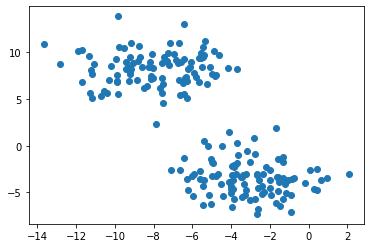
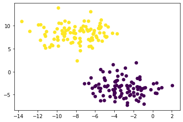
Clustering refers to the task of separating this data set into the two natural “blobs.” K-means is a very common way to achieve this task, which has good performance on circular-ish blobs like these:

from sklearn.cluster import KMeans
km = KMeans(n_clusters = 2)
km.fit(X)

plt.scatter(X[:,0], X[:,1], c = km.predict(X))

<matplotlib.collections.PathCollection at 0x23067dce550>

Harder Clustering

That was all well and good, but what if our data is “shaped weird”?

#With the seed reset (every time), the same set of numbers will appear every time
np.random.seed(1234)
n = 200
X, y = datasets.make_moons(n_samples=n, shuffle=True, noise=0.05, random_state=None)
plt.scatter(X[:,0], X[:,1])

<matplotlib.collections.PathCollection at 0x23067e2c1c0>

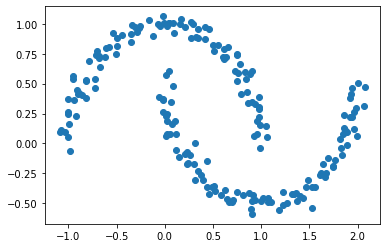
We can still make out two meaningful clusters in the data, but now they aren’t blobs but crescents. As before, the Euclidean coordinates of the data points are contained in the matrix X, while the labels of each point are contained in y. Now k-means won’t work so well, because k-means is, by design, looking for circular clusters.

km = KMeans(n_clusters = 2)
km.fit(X)
plt.scatter(X[:,0], X[:,1], c = km.predict(X))

<matplotlib.collections.PathCollection at 0x23067e83340>

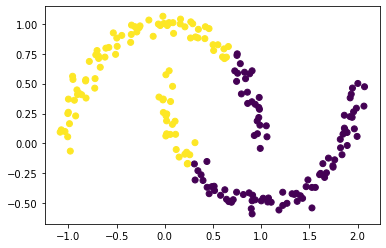
Whoops! That’s not right!

As we’ll see, spectral clustering is able to correctly cluster the two crescents. In the following steps. we will derive and implement spectral clustering.

Part A

We first construct the similarity matrix $\mathbf{A}$. $\mathbf{A}$ should be a matrix (2d np.ndarray) with shape (n, n) (recall that n is the number of data points). When constructing the similarity matrix, use a parameter epsilon.For this part, use epsilon = 0.4.

Entry A[i,j] should be equal to 1 if X[i] (the coordinates of data point i) is within distance epsilon of X[j] (the coordinates of data point j). In practical code, we test whether (X[i] - X[j])**2 < epsilon**2 for each choice of i and j. The diagonal entries A[i,i] should all be equal to zero. So here we use the function np.fill_diagonal() to set the values of the diagonal of a matrix.

since we would not want use for loop to test whether the distance satisfies the requirement for each i and j, we here use the sklearn’s pairwise_distance to efficiently calculate the distance between our data points.

from sklearn.metrics import pairwise_distances as pad
 
n = 200
ep = 0.4
p = pad(X, metric = 'euclidean')
#We first construct the *similarity matrix* (2d `np.ndarray`) with shape `(n, n)`
A = np.ndarray(shape = (n,n))
np.fill_diagonal(A, 0)
A[p<ep**2] = 1
A[p>=ep**2] = 0
A

array([[1., 0., 0., ..., 0., 0., 0.],
       [0., 1., 0., ..., 0., 0., 0.],
       [0., 0., 1., ..., 0., 0., 0.],
       ...,
       [0., 0., 0., ..., 1., 0., 1.],
       [0., 0., 0., ..., 0., 1., 0.],
       [0., 0., 0., ..., 1., 0., 1.]])

Part B

The matrix A now contains information about which points are near (within distance epsilon) which other points. We now pose the task of clustering the data points in X as the task of partitioning the rows and columns of A.

Let $d_i = \sum_{j = 1}^n a_{ij}$ be the $i$th row-sum of $\mathbf{A}$, which is also called the degree of $i$. Let $C_0$ and $C_1$ be two clusters of the data points. We assume that every data point is in either $C_0$ or $C_1$. The cluster membership as being specified by y. We think of y[i] as being the label of point i. So, if y[i] = 1, then point i (and therefore row $i$ of $\mathbf{A}$) is an element of cluster $C_1$.

The binary norm cut objective of a matrix $\mathbf{A}$ is the function

In this expression,

• $\mathbf{cut}(C_0, C_1) \equiv \sum_{i \in C_0, j \in C_1} a_{ij}$ is the cut of the clusters $C_0$ and $C_1$.
• $\mathbf{vol}(C_0) \equiv \sum_{i \in C_0}d_i$, where $d_i = \sum_{j = 1}^n a_{ij}$ is the degree of row $i$ (the total number of all other rows related to row $i$ through $A$). The volume of cluster $C_0$ is a measure of the size of the cluster.

A pair of clusters $C_0$ and $C_1$ is considered to be a “good” partition of the data when $N_{\mathbf{A}}(C_0, C_1)$ is small. To see why, let’s look at each of the two factors in this objective function separately.

B.1 The Cut Term

First, the cut term $\mathbf{cut}(C_0, C_1)$ is the number of nonzero entries in $\mathbf{A}$ that relate points in cluster $C_0$ to points in cluster $C_1$. Saying that this term should be small is the same as saying that points in $C_0$ shouldn’t usually be very close to points in $C_1$. We will write a function called cut(A,y) to compute the cut term by summing up the entries A[i,j] for each pair of points (i,j) in different clusters.

def cut(A,y):
    cut = 0
    for i in range(len(A)):
        for j in range(len(A[i])):
            if y[i] != y[j]:
                cut += A[i][j]
    return cut

Compute the cut objective for the true clusters y. Then, generate a random vector of random labels of length n, with each label equal to either 0 or 1. Check the cut objective for the random labels. You should find that the cut objective for the true labels is much smaller than the cut objective for the random labels.

This shows that this part of the cut objective indeed favors the true clusters over the random ones.

np.random.seed(1234) 
print("Cut for true labels is: ", cut(A, y))
y_random = np.random.randint(0, 2, size = n) 
print("Cur for the random labels is: ", cut(A, y_random))
# we can see that the cut objective for the true labels is much smaller than the cut objective for the random labels.

Cut for true labels is:  0.0
Cur for the random labels is:  794.0

B.2 The Volume Term

Now take a look at the second factor in the norm cut objective. This is the volume term. As mentioned above, the volume of cluster $C_0$ is a measure of how “big” cluster $C_0$ is. If we choose cluster $C_0$ to be small, then $\mathbf{vol}(C_0)$ will be small and $\frac{1}{\mathbf{vol}(C_0)}$ will be large, leading to an undesirable higher objective value.

Synthesizing, the binary normcut objective asks us to find clusters $C_0$ and $C_1$ such that:

1. There are relatively few entries of $\mathbf{A}$ that join $C_0$ and $C_1$.
2. Neither $C_0$ and $C_1$ are too small.

• We first write a function called vols(A,y) which computes the volumes of $C_0$ and $C_1$, returning them as a tuple.

• Then, we write a function called normcut(A,y) which uses cut(A,y) and vols(A,y) to compute the binary normalized cut objective of a matrix A with clustering vector y.

def vols(A,y):
    '''
    Computes the volume of each cluster
    Input: A- 2d numpy array of similarity matrix
    Input: y- a numpy array of the actual cluster data point belongs in
    Output: The volume term of cluster 0 and cluster 1 as a tuple
    '''
    v0 = np.cumsum(A,axis=0)[-1][y==0].sum()
    v1 = np.cumsum(A,axis=0)[-1][y==1].sum()
    return v0, v1

def normcut(A, y):
    # calculate our cut term
    cut_term = cut(A, y) 
    # calculate our volumes for each cluster
    v_0, v_1 = vols(A, y) 
    # Return norm cut objective
    return cut_term*(1/v_0+ 1/v_1) 

Now, we compare the normcut objective using both the true labels y and the fake labels you generated above.

np.random.seed(1234) 
print("True norm cut is: ", normcut(A, y))
print("Arbitrary norm cut is: ", normcut(A, y_random))

True norm cut is:  0.0
Arbitrary norm cut is:  1.849196291512541

We can see that the true norm cut is smaller than the arbitrary norm cut.

Part C

We have now defined a normalized cut objective which takes small values when the input clusters are (a) joined by relatively few entries in $A$ and (b) not too small. One approach to clustering is to try to find a cluster vector y such that normcut(A,y) is small. However, this is an NP-hard combinatorial optimization problem, which means that may not be possible to find the best clustering in practical time, even for relatively small data sets. We need a math trick!

Here’s the trick: define a new vector $\mathbf{z} \in \mathbb{R}^n$ such that:

Note that the signs of the elements of $\mathbf{z}$ contain all the information from $\mathbf{y}$: if $i$ is in cluster $C_0$, then $y_i = 0$ and $z_i > 0$.

Next, if you like linear algebra, you can show that

where $\mathbf{D}$ is the diagonal matrix with nonzero entries $d_{ii} = d_i$, and where $d_i = \sum_{j = 1}^n a_i$ is the degree (row-sum) from before. Here are our steps:

1. Write a function called transform(A,y) to compute the appropriate $\mathbf{z}$ vector given A and y, using the formula above.
2. Then, check the equation above that relates the matrix product to the normcut objective, by computing each side separately and checking that they are equal.
3. Check the identity $\mathbf{z}^T\mathbf{D}\mathbb{1} = 0$, where $\mathbb{1}$ is the vector of n ones (i.e. np.ones(n)). This identity effectively says that $\mathbf{z}$ should contain roughly as many positive as negative entries.

Programming Note

We can compute $\mathbf{z}^T\mathbf{D}\mathbf{z}$ as z@D@z,

Note

The equation above is exact, but computer arithmetic is not! np.isclose(a,b) is a good way to check if a is “close” to b, in the sense that they differ by less than the smallest amount that the computer is (by default) able to quantify.

def transform(A,y):
    '''
    Computes the z vector 
    Input: A, a 2d numpy array of similarity matrix, y a numpy array of the actual cluster data point belongs in
    Output: z vector, a numpy array
    '''
    v0,v1=vols(A,y)
    z = np.zeros(len(y))
    z[y==0]= 1/v0
    z[y==1]= (-1)/v1
    return z

Now we check whether the vector is valid:

# Diagonal matrix with non-zero entries d_ii = d_i where d_i is the degree
D = np.diag(A.sum(axis = 0)) 
z = transform(A, y) 
# numerator of norm cut equation
norm_cut_numer = 2 * (z @ (D - A) @ z) 
# denominator of norm cut equation
norm_cut_denom = z @ D @ z 
norm_cut_eq = norm_cut_numer/norm_cut_denom
# Check whether normcut function relates to the equation defined above by using np.isclose():
np.isclose(normcut(A, y), norm_cut_eq)

True

We check the identity:

e = np.ones(n) 

np.isclose(z @ D @ e, 0)

True

Part D

In the last part, we saw that the problem of minimizing the normcut objective is mathematically related to the problem of minimizing the function

subject to the condition $\mathbf{z}^T\mathbf{D}\mathbb{1} = 0$. It’s actually possible to bake this condition into the optimization, by substituting for $\mathbf{z}$ the orthogonal complement of $\mathbf{z}$ relative to $\mathbf{D}\mathbf{1}$. In the code below, I define an orth_obj function which handles this for you.

Use the minimize function from scipy.optimize to minimize the function orth_obj with respect to $\mathbf{z}$. Note that this computation might take a little while. Explicit optimization can be pretty slow! Give the minimizing vector a name z_.

def orth(u, v):
    return (u @ v) / (v @ v) * v

e = np.ones(n) 

d = D @ e

def orth_obj(z):
    z_o = z - orth(z, d)
    return (z_o @ (D - A) @ z_o)/(z_o @ D @ z_o)

from scipy.optimize import minimize

z_min = minimize(orth_obj, z, constraints = {'type': 'eq', 'fun': lambda z: z @ d})["x"]

Note: there’s a cheat going on here! We originally specified that the entries of $\mathbf{z}$ should take only one of two values (back in Part C), whereas now we’re allowing the entries to have any value! This means that we are no longer exactly optimizing the normcut objective, but rather an approximation. This cheat is so common that deserves a name: it is called the continuous relaxation of the normcut problem.

Part E

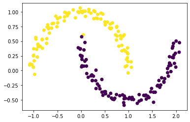
Recall that, by design, only the sign of z_min[i] actually contains information about the cluster label of data point i. Plot the original data, using one color for points such that z_min[i] < 0 and another color for points such that z_min[i] >= 0.

Does it look like we came close to correctly clustering the data?

plt.scatter(X[:,0], X[:,1], c = np.where(z_min < 0, 0, 1))

<matplotlib.collections.PathCollection at 0x23067ef3100>

Part F

Explicitly optimizing the orthogonal objective is way too slow to be practical. If spectral clustering required that we do this each time, no one would use it.

The reason that spectral clustering actually matters, and indeed the reason that spectral clustering is called spectral clustering, is that we can actually solve the problem from Part E using eigenvalues and eigenvectors of matrices.

Recall that what we would like to do is minimize the function

with respect to $\mathbf{z}$, subject to the condition $\mathbf{z}^T\mathbf{D}\mathbb{1} = 0$.

The Rayleigh-Ritz Theorem states that the minimizing $\mathbf{z}$ must be the solution with smallest eigenvalue of the generalized eigenvalue problem

which is equivalent to the standard eigenvalue problem

Why is this helpful? Well, $\mathbb{1}$ is actually the eigenvector with smallest eigenvalue of the matrix $\mathbf{D}^{-1}(\mathbf{D} - \mathbf{A})$.

So, the vector $\mathbf{z}$ that we want must be the eigenvector with the second-smallest eigenvalue.

In the following codes, we construct the matrix $\mathbf{L} = \mathbf{D}^{-1}(\mathbf{D} - \mathbf{A})$, which is often called the (normalized) Laplacian matrix of the similarity matrix $\mathbf{A}$. Find the eigenvector corresponding to its second-smallest eigenvalue, and call it z_eig. Then, plot the data again, using the sign of z_eig as the color.

L = np.linalg.inv(D) @ (D - A)
ev, U = np.linalg.eig(L)
ev_sort = ev.argsort() 
z_eig = U[:,ev_sort][:,1]

plt.scatter(X[:,0], X[:,1], c = np.where(z_eig < 0, 0, 1))

<matplotlib.collections.PathCollection at 0x23067f4b3a0>

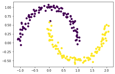
In fact, z_eig should be proportional to z_min, although this won’t be exact because minimization has limited precision by default.

Part G

We now write a function called spectral_clustering(X, epsilon) which takes in the input data X (in the same format as Part A) and the distance threshold epsilon and performs spectral clustering, returning an array of binary labels indicating whether data point i is in group 0 or group 1.

Outline

Given data, we need to:

1. Construct the similarity matrix.
2. Construct the Laplacian matrix.
3. Compute the eigenvector with second-smallest eigenvalue of the Laplacian matrix.
4. Return labels based on this eigenvector.

def spectral_clustering(X, epsilon):
    """
    1. We first create an empty similarity matrix A with shape n x n,and the matrix noting (X[i] - X[j])**2
    2. We then modify our similarity matrix to be 1 if it's within our epsilon and 0 if not on the diagonal
    
    Note:
    a. D is the diagonal matrix with nonzero entries 
    b. L is normalized Laplacian matrix using pseudoinverse of D
    c. ev:eigenvalues, U:eigenvectors 
    d. ev_sort:eigenvalues sorted
    e. z_eig gives the eigenvector associated to the second-smallest eigenvector
    
    3. we return labels using eigenvector above with those with negative values in C_0, positive values in C_1
    """
    # Creates an empty n x n matrix
    A = np.ndarray(shape = (X.shape[0], X.shape[0])) 
    # Distance matrix from data set X
    P = pad(X, metric = 'euclidean') 
    # If value of distance matrix is within chosen epsilon, entry = 1
    A[P < epsilon**2] = 1 
    # If value of distance matrix is greater than chosen epsilon, entry = 0
    A[P >= epsilon**2] = 0 
    # Diagonal entries are 0
    np.fill_diagonal(A, 0) 
    
    D = np.diag(A.sum(axis = 0)) 
    L = np.linalg.pinv(D) @ (D - A)
    
    ev, U = np.linalg.eig(L)
    ev_sort = ev.argsort()  
    z_eig = U[:,ev_sort][:,1]
    
    return np.where(z_eig < 0, 0, 1)

Part H

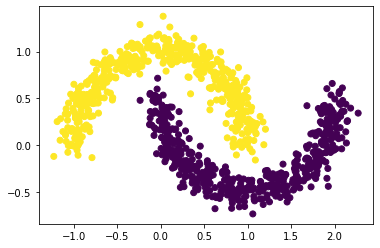
We now run a few experiments using our function, by generating different data sets using make_moons. We try to see what happens when we increase the noise. Does spectral clustering still find the two half-moon clusters? For these experiments, we can increase n to 1000.

np.random.seed(7726) #Set seed for reproducibility
# The number of data points 
n2 = 1000 
X2, y2 = datasets.make_moons(n_samples=n2, shuffle=True, noise=0.1, random_state=None)
# Creates label vector
z2 = spectral_clustering(X2, epsilon = 0.45) 
plt.scatter(X2[:,0], X2[:,1], c = z2) # Plots it

<matplotlib.collections.PathCollection at 0x23067fa4df0>

n = 1000
NOISE = 0.2
X, y = datasets.make_moons(n_samples=n, shuffle=True, noise=NOISE, random_state=None)
clusterLabels = spectral_clustering(X, epsilon = 0.4)
plt.scatter(X[:,0], X[:,1], c = clusterLabels)

<matplotlib.collections.PathCollection at 0x23067ffe220>

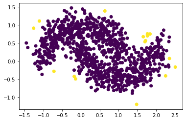
We can see that noise reates more random data and less clear distinctions between clusters

Part I

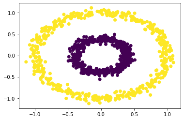
Now we tru spectral clustering function on another data set – the bull’s eye!

np.random.seed(1234)

n = 1000
X, y = datasets.make_circles(n_samples=n, shuffle=True, noise=0.05, random_state=None, factor = 0.4)
plt.scatter(X[:,0], X[:,1])

<matplotlib.collections.PathCollection at 0x2306804ad30>

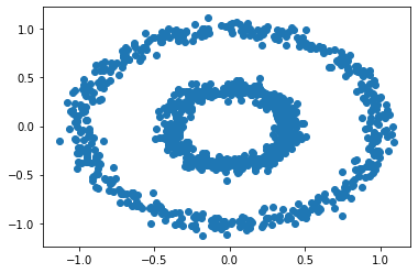
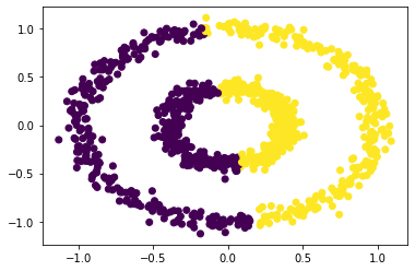
There are two concentric circles. As before k-means will not do well here at all.

km = KMeans(n_clusters = 2)
km.fit(X)
plt.scatter(X[:,0], X[:,1], c = km.predict(X))

<matplotlib.collections.PathCollection at 0x2306809aa30>

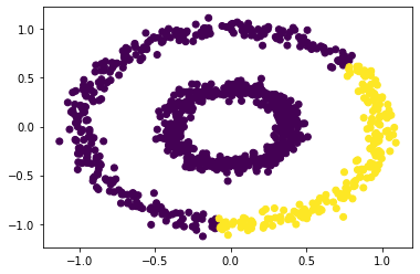
To test whether our function can successfully separate the two circles, we need some experimentation here with the value of epsilon. We rry values of epsilon between 0 and 1.0.

plt.scatter(X[:,0], X[:,1], c = spectral_clustering(X, 1)) 

<matplotlib.collections.PathCollection at 0x230680e5f70>

plt.scatter(X[:,0], X[:,1], c = spectral_clustering(X, 0.1)) 

<matplotlib.collections.PathCollection at 0x2306813b760>

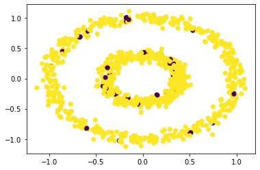
We can see that for epsilon = 0.1 or 1, if does not do a great clustering. Thus we try some values in between.

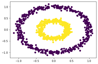
plt.scatter(X[:,0], X[:,1], c = spectral_clustering(X, 0.5)) 

<matplotlib.collections.PathCollection at 0x23068186ee0>

plt.scatter(X[:,0], X[:,1], c = spectral_clustering(X, 0.6)) 

<matplotlib.collections.PathCollection at 0x230681dc670>

plt.scatter(X[:,0], X[:,1], c = spectral_clustering(X, 0.7)) 

<matplotlib.collections.PathCollection at 0x23068228df0>

plt.scatter(X[:,0], X[:,1], c = spectral_clustering(X, 0.4)) 

<matplotlib.collections.PathCollection at 0x2306827c580>

plt.scatter(X[:,0], X[:,1], c = spectral_clustering(X, 0.8)) 

<matplotlib.collections.PathCollection at 0x230682c8a60>

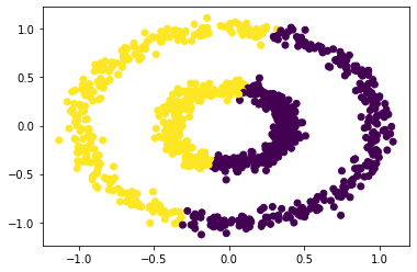
We can see that when epsilson is in between 0.5 and 0.7, we could have clear separations. For values below the range or higher the range, it fails to have the clustering effect.